
1 Introduction
As the conversation about systemic sexism and gender bias grows, research on the existence of a wage gap becomes increasingly crucial. Economists such as Claudia Goldin, Francine Blau, and Lawrence Katz have conducted extensive studies investigating the factors contributing to the wage gap, exploring issues related to gender, labor markets, and policies affecting income differentials. Institutions like the World Bank, OECD (Organisation for Economic Co-operation and Development), and the Institute for Womens Policy Research have also generated comprehensive reports and analyses, shedding light on global and national trends in gender pay gaps, highlighting disparities across different countries, industries, and demographic segments. Additionally, advocacy groups like the American Association of University Women (AAUW) and Catalyst have produced research focusing on gender inequalities in pay and employment practices, advocating for policy changes and workplace reforms to address these disparities [1]. In our investigation, we delve into the impact of gender on salary and income levels through a machine-learning data analysis approach. Leveraging the power of techniques such as random forest classifiers and regression, we aim to discern whether there exists a correlation between gender and earnings.
As We use the dataset “Glassdoor- Analyze Gender Pay Gap” provided by Kaggle.com to perform our analysis. We note that this dataset is relatively small and any results gathered from our study may not be able to generalize to broad statements about the wage gap and gender discrimination in the workplace. However, by analyzing one dataset, we seek to uncover patterns, dependencies, and potential biases that might manifest in salary distributions across genders. Through this analysis, we aspire to contribute empirical evidence to the ongoing discourse surrounding gender-based income inequalities, offering insights that could inform policy initiatives and organizational strategies toward fostering greater fairness and equity in remuneration practices.
2 Data Visualization
In our project, we began by loading the Glassdoor Gender Pay Gap dataset from Kaggle.com using pandas. The dataset is composed of data about employees from one company. The data is anonymous and reported by the anonymous-company so this creates no ethical issues or doubt in the trustworthiness of the data.
A significant addition to our preprocessing was the combination of BasePay and Bonus columns, followed by normalizing this combined pay. This ensured that our analyses and models considered total earnings rather than just base pay or bonuses separately. By normalizing this combined value, we maintain consistency across different scales of pay and bonus values, allowing for a more accurate comparison and analysis.
We also employed label encoding for categorical data such as JobTitle, Gender, Education, Dept, and Seniority, converting them into numerical values for computational efficiency. This step was vital as most algorithms require numerical input for effective analysis. The dataset, now with normalized pay values and encoded categorical variables, is well-prepared for rigorous statistical analysis and machine learning modeling, ensuring accuracy and reliability in our subsequent analyses and predictions.
Our dataset came with no missing values. This allowed for minimal data cleaning. We decided to proceed with these features to observe if the gender pay gap is observable with basic information that would be considered by employers when considering salaries.
3 Analysis/Visualizations
3.1 Visualization of Data
Before diving into the deep-end of regression and classification, we want to visualize aspects of the dataset that we found interesting. The first characteristic of the data we want to emphasize is the distribution of men and women in each job title.
job_bar_graph()
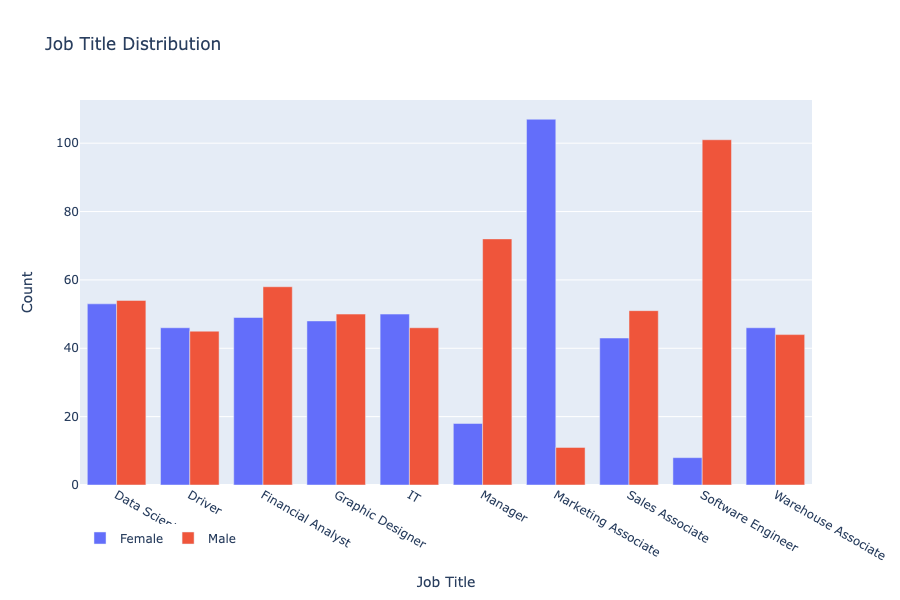
We see that for the majority of job titles, there are approximately the same amount of men and women in those positions. However, there exist some jobs where the distribution of gender is heavily skewed, such as marketing associate, software engineer, and manager. While our dataset is too small to draw any conclusions about societal trends, we can conclude that not all positions at this company are equal in distribution of gender.
Another visual that we found important for the analysis of our data is comparison of pay between the genders in each job title. Below we visualize a bar graph where we show the difference between the average male total pay and average female total pay (male - female) for each position.
salary_difference()
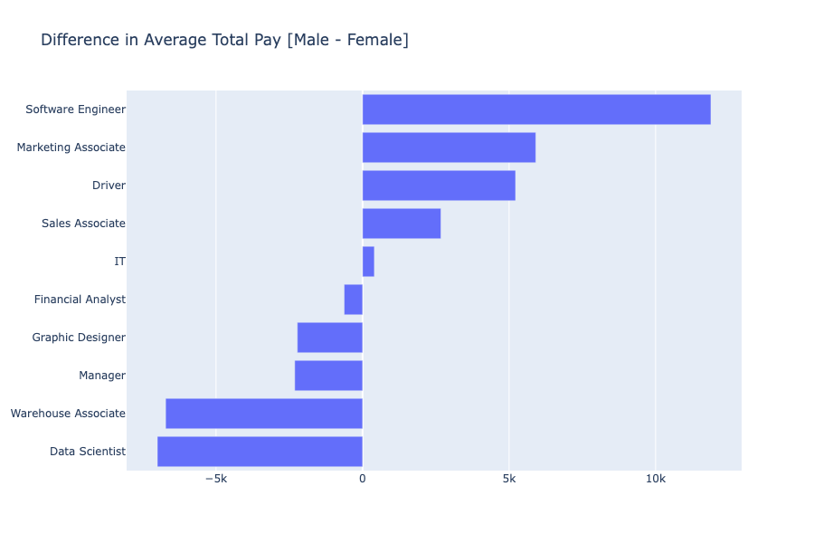
Being below the average pay of the opposite gender exists for both men and women as seen above. There are some positions where the average male employee make more and some positions where the average female employee makes more. While this graph may appear to answer the original question of the existence of the gender pay graph, we recognize that salary is more complex than just job titles and genders. In the following sections we analyze the other variables that come into play and their importances.
3.2 Education Analysis
To observe the effects that gender has on pay, we analyze subsets of the original dataset grouping by education levels. To begin this analysis we provide a visual of the distributions of gender by education level.
distribution_show(df,label_encoder_education,"Education")
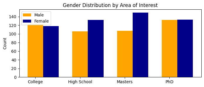
This bar graph depicts the counts of men and women in each education level in our dataset. We see that each education level has more than 100 data points for both genders. Likewise, we observe that in this dataset the distribution of men and women is roughly equal. We want to make note that we provide this visual to provide a more-detailed glimpse into our dataset and we will not conduct an analysis of gender diversity in education. While that would be an interesting subject, it would require a larger dataset and more knowledge about the sampling techniques used to make any reasonable conclusions.
As described above, to analyze the effects that gender plays in pay we used regression models to view the significance of the features and w gender compares. After breaking the data down by education levels and performing gridsearches for the optimal hyperparameters, the results of the random forest regressor, boosted gradient regressor, and xgboost regressor for education are below:
Education Regression Mean Squared Errors
| H.S | College | Masters | PhD | |
|---|---|---|---|---|
| RFR | 0.00463 | 0.00728 | 0.00624 | 0.00753 |
| GBR | 0.00464 | 0.00573 | 0.00646 | 0.00615 |
| XGBR | 0.00303 | 0.00443 | 0.00465 | 0.00437 |
Looking at the table, we can see that the xgboost regressor achieved the lowest mean square errors. For the purposes of this paper, we will analyze the most important features for this model. The ranked features are listed for each education level in the table below.
Feature Importance
| Ranking | H.S | College | Masters | PhD |
|---|---|---|---|---|
| 1 | Seniority: 0.44 | Seniority: 0.29 | Seniority: 0.55 | Seniority: 0.47 |
| 2 | Age: 0.27 | Gender: 0.17 | Age: 0.20 | Age: 0.27 |
| 3 | Job title: 0.13 | Job Title: 0.12 | Gender: 0.10 | Job Title: 0.17 |
We can see that gender is never the most important feature to estimate. Likewise, it is very rare for gender to have importance greater than 0.1 with college and masters being the only education levels with gender as an important features.
Now moving onto classification. We sought to classify an employee's gender and analyze which features are most important. We performed gridsearches on the random forest, boosted gradient, and xgboost classifierusing the same datasets for each. From there, we analyzed the results. The accuracies for each model are displayed below.
Education Classification Accuracy
| H.S | College | Masters | PhD | |
|---|---|---|---|---|
| RFC | 0.58 | 0.69 | 0.58 | 0.54 |
| GBC | 0.62 | 0.67 | 0.54 | 0.60 |
| XGBC | 0.64 | 0.73 | 0.58 | 0.62 |
Once again, the xgboost provided the best results. Below, we display the most important features of that model and their significances.
Feature Importance
| Ranking | H.S | College | Masters | PhD |
|---|---|---|---|---|
| 1 | Job title: 0.30 | Base Pay: 0.21 | Base Pay: 0.20 | Dept.: 0.18 |
| 2 | Age: 0.16 | Dept.: 0.16 | Job Title: 0.17 | Seniority: 0.18 |
| 3 | Base Pay: 0.13 | Age: 0.15 | Bonus: 0.13 | Job Title: 0.17 |
Before we dive into the analysis, we want to make one note. Originally, we dropped base pay and bonus as features, replacing them with normalized pay. However, after comparison, the classification results did better with base pay and bonus in the dataset versus normalized pay. This is solely for this section and the dataset will return to as previously described in the following sections.
From these classifiers, we see that base pay and bonuses consistently are important features in classifying between genders, especially those with college degrees. Between the college pay regressor and gender classifier having gender and base pay in their most important features, respectively, and accuracte results, we can conclude there is some form of pay disparity between the genders at the college level.
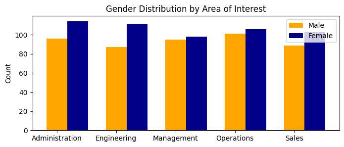
3.3 Department Analysis
We next focus in on differences in pay among different department levels. There are 5 different departments: Administration, Engineering, Management, Operations, and Sales. We look first at the gender distribution in each department, displayed as a histogram. Then we use random forests, gradient boosting, and xgboost to examine the most important features in the regressors and classifiers.
distribution_show(df,label_encoder_dept,"Dept")
Department Regression Mean Squared Errors
| Operations | Management | Administration | Sales | Engineering | |
|---|---|---|---|---|---|
| RFR | 0.00976 | 0.0100 | 0.00789 | 0.00653 | 0.01056 |
| GBR | 0.0116 | 0.00529 | 0.00709 | 0.00600 | 0.0090 |
| XGBR | 0.00489 | 0.0047 | 0.00398 | 0.00448 | 0.0036 |
Since XGBR had the lowest Mean Squared Error for every department, we analyze the results of that regression.
Feature Importance of Departments using XGBoost Regression
| Ranking | Operations | Management | Administration | Sales | Engineering |
|---|---|---|---|---|---|
| 1 | Age: 0.41 | Seniority: 0.40 | Seniority: 0.51 | Seniority: 0.46 | Seniority: 0.50 |
| 2 | Seniority: 0.35 | Age: 0.27 | Age: 0.16 | Age: 0.25 | Age: 0.22 |
| 3 | Job Title: 0.14 | Job Title: 0.14 | Gender: 0.11 |
Notice that Seniority, Age, and Job Title seem to be important features in determining Salary for an individual. Gender only appears as an important feature in the Sales department. Thus we can conclude that Gender is not a primary feature when determining salary in specific departments.
Classification Accuracy of Departments
| Operations | Management | Administration | Sales | Engineering | |
|---|---|---|---|---|---|
| RFC | 0.57 | 0.62 | 0.41 | 0.61 | 0.62 |
| GBC | 0.62 | 0.53 | 0.51 | 0.67 | 0.56 |
| XGBC | 0.67 | 0.62 | 0.42 | 0.64 | 0.51 |
We will examine the most important features of XGBoost on Operations and Management, Gradient Boost on Administration and Sales, and Random Forest on Engineering because these provide the highest accuracy.
Feature Importance of Departments using XGBoost Regression
| Ranking | Operations | Management | Administration | Sales | Engineering |
|---|---|---|---|---|---|
| 1 | Seniority: 0.23 | Job Title: 0.28 | NormComp: 0.38 | NormComp: 0.30 | NormComp: 0.26/td> |
| 2 | PerfEval: 0.17 | NormComp: 0.22 | Age: 0.23 | Job Title: 0.30 | Age: 0.24 |
| 3 | Job Title: 0.17 | Age: 0.16 | Age: 0.22 | Job Title: 0.18 |
Note that the accuracy for each of these departments is slightly above 0.5, meaning that predicting gender using classification trees is slightly better than random. The most important features in predicting gender tend to be NormalizedTotalComp, Job Title, and Age. This means that total compensation is an important feature in predicting gender, but we must avoid extrapolating to claim this is evidence of the wage gap. We recognize that there may be other societal factors such as education, seniority, or age that may result in a lower compensation for an women in the workplace. In other words, if we claim that Total Compensation being an important feature in predicting gender is evidence of the wage gap, we are forgetting that different compensation between men and women may be a result of different education levels, job titles, or seniority levels, and those areas should be further examined to make a strong conclusion about the wage gap.
3.4 Complete Dataset Analysis
After performing the analyses above on different subsets of the data, we sought to observe the gender pay gap from a more holistic view, using the whole dataset. To save space, we have condensed the results into tables below but the results can be replicated using the code found in the attached .py file. Beginning with classification the accuracies and most important features of each algorithm are displayed below:
Classification Results On Complete Dataset
| Classifier | Accuracy |
|---|---|
| RFC | 0.68 |
| GBC | 0.65 |
| XGBC | 0.69 |
XGBC Most Important Features
| Feature | Importance |
|---|---|
| Job Title | 0.49 |
| NormPay | 0.14 |
| Age | 0.13 |
We see that every classifier did better then randomly guessing, with XGBC having the best results. For the classification problem, the normalized total pay was the second most important feature.
Below are the results from using regression to predict normalized pay.
Regression Results On Complete Dataset
| Regressor | MSE |
|---|---|
| RFR | 0.0048 |
| GBR | 0.0048 |
| XGBR | 0.0029 |
XGBR Most Important Features
| Feature | Importance |
|---|---|
| Seniority | 0.52 |
| Age | 0.19 |
| Job Title | 0.13 |
We see that gender was not one of the top three most important features. Gender had an importance of approximately 0.09. This would make sense as gender would play a minor part in pay under the assumptions of the gender pay gap. Other features such as job title and seniority make sense in establishing pay as those are more connected with one’s duties and loyalty to the company.
While these results do provide some evidence into a disparity in pay between the genders, there is no solid way to establish which way this disparity goes. To establish the direction of the disparity, we would have to analyze the spits at each node, which isn’t feasible.
3.5 OLS Analysis
In our comprehensive analysis of the gender pay gap, we conducted ordinary least squares (OLS) regression analysis to quantitatively measure the effects of various factors on normalized total compensation. This study complements our previous machine learning models and provides a clearer mathematical perspective on the variables affecting earnings levels. Below is a simplistic OLS model that uses job title, gender, age, performance evaluation, education, department, and seniority as independent variables to estimate the dependent variable of normalized compensation.
                             OLS Regression Results
===============================================================================
Dep. Variable:     NormalizedTotalComp   R-squared:                       0.633
Model:                             OLS   Adj. R-squared:                  0.631
Method:                  Least Squares   F-statistic:                     343.2
Date:                 Wed, 06 Dec 2023   Prob (F-statistic):          1.33e-213
Time:                         03:15:04   Log-Likelihood:                 1073.0
No. Observations:                 1000   AIC:                            -2134.
Df Residuals:                      994   BIC:                            -2104.
Df Model:                            5
Covariance Type:             nonrobust
==============================================================================
                 coef    std err          t      P>|t|      [0.025      0.975]
------------------------------------------------------------------------------
const          0.1640      0.012     14.176      0.000       0.141       0.187
Gender         0.0521      0.005      9.848      0.000       0.042       0.062
Age            0.0053      0.000     28.611      0.000       0.005       0.006
PerfEval       0.0040      0.002      2.138      0.033       0.000       0.008
Education      0.0142      0.002      5.924      0.000       0.009       0.019
Seniority      0.0536      0.002     28.418      0.000       0.050       0.057
==============================================================================
Omnibus:                       30.419   Durbin-Watson:                   1.957
Prob(Omnibus):                  0.000   Jarque-Bera (JB):               32.405
Skew:                           0.427   Prob(JB):                     9.19e-08
Kurtosis:                       3.216   Cond. No.                         196.
==============================================================================

Notes:
[1] Standard Errors assume that the covariance matrix of the errors is correctly specified.
The model's R-squared value of 0.637 explains 63.7% of the variation in compensation. The model results also indicate that Gender significantly correlates to compensation, with a 5.11% increase for a specific gender. The model also indicates that Job Title, Age, and Seniority also impact compensation, with Seniority having a strong positive relationship with each additional year leading to a 0.53% increase in compensation. Performance Evaluation and Education have smaller but significant effects (0.0040 and 0.0143), influencing compensation. Departmental variations in compensation exist (0.0043 coefficient), but they are less significant than Seniority and Gender.
This analysis confirms the influence of Gender and highlights the role of Age, Seniority, Job Title, Education, and Department in compensation. However, this analysis's limitations and critiques go beyond the complex dynamics that influence compensation. The primary critique is that several variables included in this regression are encoded data. This is more acceptable in ordinal data points, such as Education levels, where the assigned integers reflect the value of the assignment. However, in our encodings of nominal data points, such as Job Title and department, the assigned integer value has no real meaning in its assignment.
While this basic OLS model sheds light on critical factors affecting wages, its limitations highlight the need for a more informative and nuanced approach. To address this, we turn to quantile regression, which allows us to examine how these variables' impacts vary across different income distributions and better understand the underlying trends in compensation disparities.
Quantile Regression Coefficients
| 0.25 | 0.5 | 0.75 | |
|---|---|---|---|
| Intercept | 0.084456 | 0.137970 | 0.195391 |
| Gender | 0.046265 | 0.042455 | 0.042948 |
| JobTitle | 0.000267 | 0.002806 | 0.003955 |
| Age | 0.005184 | 0.005352 | 0.005235 |
| PerfEval | 0.008591 | 0.003362 | 0.002428 |
| Education | 0.011199 | 0.016336 | 0.016012 |
| Dept | 0.005535 | 0.004135 | 0.003120 |
| Seniority | 0.056841 | 0.053406 | 0.054394 |
In our quantile analysis, we aimed to assess how various factors influence normalized total compensation across different income percentiles (25th, 50th, 75th), offering a more nuanced view of wage dynamics. Gender was consistently influential across all percentiles, with coefficients of 0.0463 at the 25th percentile, 0.0425 at the median (50th percentile), and 0.0429 at the 75th percentile. In contrast, the impact of Job Title strengthens as income rises, with coefficients ranging from 0.0003 to 0.0040 across percentiles. Meanwhile, Seniority, Age, and Education maintain their influence across percentiles, providing stability in compensation dynamics. Notably, the significance of Performance Evaluation peaks at the 25th percentile with a coefficient of 0.0086 but diminishes as income increases. This intricate analysis shows the varied nature of income disparities. While illuminating, it is important to acknowledge that our approach has limitations inherent to the dataset and methodology, suggesting potential for further research exploring additional factors and advanced statistical techniques.
Conclusion
Our comprehensive analysis, centered on exploring the impact of gender on salary and income levels, has yielded significant insights, shedding light on the intricacies of the gender wage gap. By meticulously applying machine learning techniques such as Random Forest Classifiers and Regressors, Gradient Boosting, and XGBoost, along with the application of Ordinary Least Squares (OLS) regression, we have untangled critical dimensions of this socio-economic issue.
Our findings indicate that factors like job title, education, department, seniority, and age play substantial roles in determining income levels, with gender being particularly impactful. The OLS regression results, with a notable R-squared value, emphasize that a significant portion of compensation variability can be attributed to these variables. This not only substantiates our initial hypothesis but also echoes the broader academic understanding of the wage gap.
In line with the project objectives, we have sought to answer our research questions using data analytics and machine learning techniques, providing a nuanced understanding of the factors influencing the wage gap. Our study, while limited by the scope of the data, offers a lens through which the complex nature of gender-based income disparities can be viewed, highlighting areas where policy and organizational reforms or advocacy could be most impactful.
As we conclude, we recognize the limitations inherent in our analysis, particularly regarding the dataset's scope and potential biases. Future research could build on our findings by incorporating a more diverse and extensive dataset, offering a more exhaustive view of the gender pay gap across different sectors and regions. Ultimately, our project stands as a testament to the power of data analytics and machine learning in dissecting and understanding complex socio-economic issues. It offers a data-driven foundation for further academic inquiry and informs potential policy-making, aiming to foster a more equitable and just society.
Ethics
As mentioned before, we do not belived that generalizations about this research can be drawn to provide a final answer to the question of the gender pay gap. However, we do believe that this research contributes to the conversation. We hoped to provide results that could further inform employers and managers to promote equality in the workplace. We also hope that the results of this study will be used responsibly and ethically and that our work will inspire others to research further into the existence of a gender wage gap.
References
[1] Wikimedia Foundation. (2023, December 14). Gender pay gap. Wikipedia.