Abstract
Classical conditioning, a foundational concept in psychology, involves the formation of associations between stimuli and responses. Our study examines how the strength of associations between conditioned stimuli and responses changes over time. Drawing inspiration from the work of Pavlov and Rescorla-Wagner, our exploration builds on classical conditioning principles. By delving into the dynamics of associative strength, this research contributes to a deeper understanding of how organisms form and modify conditioned responses, offering insights into the malleability of learned associations.
1 Background/Motivation
Classical conditioning is one of the most significant psychological findings influencing how humans perceive themselves, their behavior, and their learning processes. There are four key terms in classical conditioning: the conditioned stimulus (CS): a neutral stimulus like a bell’s sound; the unconditioned stimulus (US): a biologically potent trigger like the taste of food; the unconditioned response (UR): an innate reflex response, such as salivation; and the conditioned response (CR): a reaction to the CS when presented in isolation [1]. We will look at ways to model the associative strength between a CS and its CR within a vacuum where CS and US are the only stimuli present. The foundation of our model will be the Rescorla–Wagner model, which is a relatively simple and common model used in classical conditioning. We will also investigate the effects of varying inter-stimulus-intervals (ISI), which is the time difference between introducing the CS and introducing the US [2].
It is also important to understand the difference between acquisition and extinction trials. An acquisition trial is one in which the CS is paired with the US, strengthening the relationship between the CS and the CR. An extinction trial is one in which only the CS is used, which weakens the relationship between the CS and the CR [2].
1.1. Related Work
Pavlov is mainly credited with his early research of classical conditioning. Pavlov’s experiments tested dogs’ association of a bell sound (CS) with the taste of food (US) to salivation (CR).
In the early 1970s, Robert Rescorla and Allan Wagner formalized Pavlov’s research by developing a model of classical conditioning known as the Rescorla-Wagner model, which aimed to explain the cognitive processes underlying associative learning. We build upon their model to analyze the effects of the ISI and further investigate the acquisition and extinction trials [1].
1.2. Building on Previous Work>
Our modifications to the Rescorla-Wagner model aim to enhance its realism and applicability in simulating real-world learning processes. We have made the following significant improvements:
- Transition to a Continuous Model:
- Rationale: The original model’s discrete approach oversimplifies the learning process, ignoring the continuous and gradual nature of how organisms learn and adapt. Continuous modeling aligns more closely with the fluidity of real-world learning and memory formation.
- Improvement: This shift allows for a more granular and accurate depiction of the learning curve. It facilitates the examination of learning dynamics at any given point in time, providing a richer understanding of the nuances in associative strength development.
- Modified Lambda Function for Extinction Trials:
- Rationale: The original model’s binary treatment of lambda during extinction trials does not capture the gradual diminishment of associative strength. Realistically, learned associations fade over time, influenced by factors like the strength of initial learning, frequency of reinforcement, and time elapsed since the last reinforcement.
- Improvement: Our model’s time-dependent lambda accounts for these factors, offering a more nuanced view of extinction. This approach reflects the complexity of how memory and learned associations degrade, particularly in scenarios where stimuli are no longer paired.
- Inclusion of Inter-Stimulus Interval (ISI) Consideration:
- Rationale: The timing between the conditioned stimulus (CS) and unconditioned stimulus (US) is a critical factor in learning, with significant implications for the strength and speed of association formation. The original model’s lack of ISI consideration fails to account for these temporal dynamics, which are crucial in conditioning.
- Improvement: By integrating ISI into our model, we can explore how different intervals impact learning. This addition is particularly relevant for understanding the conditions under which rapid learning occurs, as well as scenarios where delayed pairing leads to weaker or more complex associative patterns.
These enhancements collectively extend the scope and depth of the Rescorla-Wagner model. By introducing a continuous framework, incorporating a dynamic lambda for extinction, and considering the impact of ISI, our model provides a more comprehensive and realistic tool for examining classical conditioning in a variety of contexts.
2 Modeling
In order to understand the modeling choices in our model of classical conditioning, it is helpful to first look at the original Rescorla-Wagner model. The original model is as follows:
\[ \Delta V = \alpha \cdot \beta \cdot (\lambda - \Sigma V) \] where \(\alpha\) is the saliency of the CS, \(\beta\) is the learning rate of the US, and \(\lambda \in \{0, 1\}\) is a parameter that determines whether this trial is an acquisition or extinction trial, and \(\Sigma V\) is the total stimuli present [3].
2.1 Continuity
The original model is discrete by construction. We modify this model to a continuous state by considering the time derivative \(\frac{d}{dt}V\) and treating it as a logistic growth equation. Thus, in our new model, \(\lambda\) will be a function of time (\(t\)) to fit continuity and for accuracy of real-world problems. This continuous model will allow us to apply continuous ODE methods to this problem. Our basic continuous model is as follows:
\( \begin{equation} \frac{dV}{dt} = \alpha \cdot \beta \cdot (\lambda(t) - V) \tag{1} \end{equation} \)
2.2 Modification to Extinction Trials
In the original model, \(\lambda = 0\) whenever the trial is an extinction trial. We modify \(\lambda\) to still consider important factors such as saliency, memory of the test subject, and learning rate even during an extinction trial.
In our updated model, \(\lambda\) is a function of time (\(t\)) and is defined as follows:
\( \begin{equation} \lambda(t) = \begin{cases} \gamma \cdot \alpha \cdot \beta \cdot (t - \epsilon) + 1 & t \geq \epsilon \\ 1 & t < \epsilon \end{cases} \tag{2} \end{equation} \)
\(\gamma\) is a constant that represents the memory capacity of the test subject. For example, a human will have a stronger ability to recall than a fish. We assume that \(\gamma\) is constant for the test subject for our exploration. \(\epsilon\) is the time when the US is removed from the trial sequence.
Consider a Pavlov example with a test subject as a dog where the CS is a bell, the US is the smell of food, and the CR is salivation. At the beginning of the trial sequence, the bell and the smell of food will be paired together for the acquisition trials. In these trials, \(\lambda(t)=1\) because \(t < \epsilon\). However, as soon as the smell of food is removed from the trial sequence, we are at time ε, so all subsequent trials will contain a \(\lambda\) parameter that is a function of the dog’s memory, the salience of the bell, and the learning rate of the dog.
We went with our definition of \(\lambda\) to test a state in which the subject is highly dependent on the CS. A CS such as electroshock will produce a higher value \(\beta\). When \(\beta\) is higher, the associative strength grows at a faster rate. We believe this leads to the subject being dependent on a stimulating CS. When the US, the food, is presented without the CS, we would expect this dependence to backfire and the associative strength to decrease at a faster rate due to the large \(\beta\).
2.3 Consideration of the ISI
The inter-stimulus-interval (ISI), or the time difference between introducing the CS and introducing the US, is an important factor to consider in our model as well. We incorporate the ISI into our model as follows:
\( \begin{equation} \frac{dV}{dt} = \alpha \cdot (ISI_{modifier} \cdot \beta) \cdot (\lambda(t) - V) \tag{3} \end{equation} \)
where the \( ISI_{modifier} \) is given by
\[ ISI_{modifier} = 1 - \frac{ISI}{2 \cdot ISI_{max}} \]
This factor causes the learning rate to decrease more as the \( ISI \) approaches \( ISI_{max} \). So, if the US and CS coincide, it is pure Hebbian learning, requiring no ‘conscious observation,’ therefore, the likelihood of learning is significantly larger than if US and CS do not coincide, which requires ‘conscious observation’ and is, therefore, less likely to occur.
3 Results
3.1 Rescorla-Wagner Results
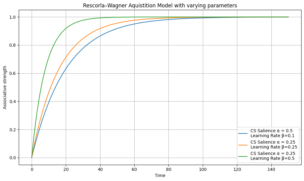
In order to understand the way our modifications impact the modeling of classical conditioning, we provide the results of the continuous Rescorla-Wagner model (Eq. 1) as a baseline. With the basic model, one is able to vary two parameters–the saliency (\( \alpha \)) and the learning rate (\( \beta \)). These inputs alter the rate at which the associative strength increases over time, as seen below:

Figure 1. Associative Strength Modeled by Eq. 1
This model considers the experiment in which the US is never removed, and the subject is never given an opportunity to forget the association. This provides results similar to what would be observed with logistic growth, where the associative strength approaches the maximum associative strength, \(\lambda\).
3.2 Extinction Model
In the extinction model (Eq. 1,2), we modify the constant \( \lambda \) to be a function of time. This update in lambda considers the decay of the maximum associative strength over time. In the context of Pavlov’s experiments, this represents the removal of the US (the food) after a specific time. The removal of the US alters the classical conditioning of the dog by presenting the CS (the bell) without the US (the food), leading to a decay in the maximum associative strength.
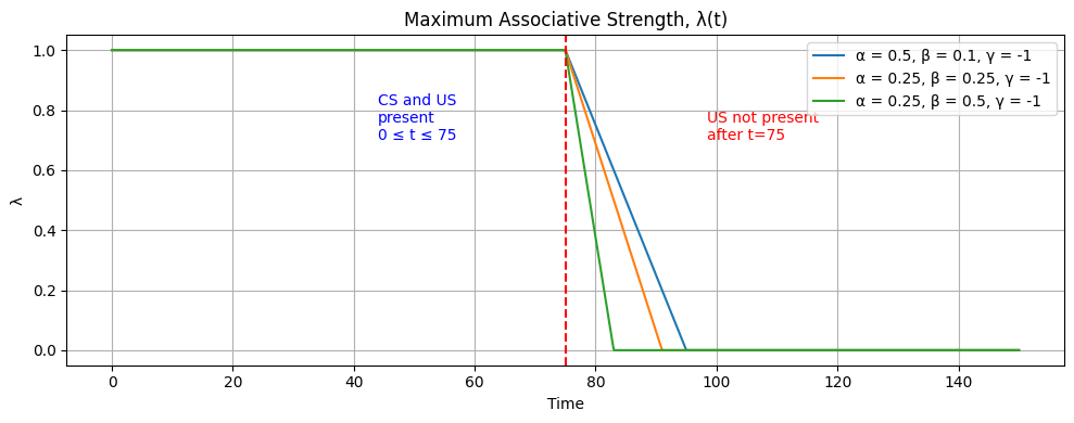
As described in Section 2.2, \( \lambda(t) \) is modeled with some consideration of the saliency (\( \beta) \), the learning rate (\( \alpha) \),, and the subject’s biological ability to forget \( (\gamma) \). In our trials, \( \gamma \) will remain constant. Below, we model the effects different combinations of \( \beta \) and \( \alpha \) have on the rate of decay of the maximum associative strength after removing the US at \( t = 75 \).

Figure 2. \( \lambda (t) \) with varying \( \alpha \) and \( \beta \) and fixed \( \gamma \)
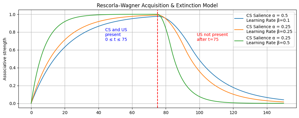
Including this update of \( \lambda \), affects the modeling of the associative strength as seen in Figure 3.

Figure 3. Updated version of the Recsorla-Wagner model considering \( \lambda (t) \)
3.3 Extinction + ISI Model Results
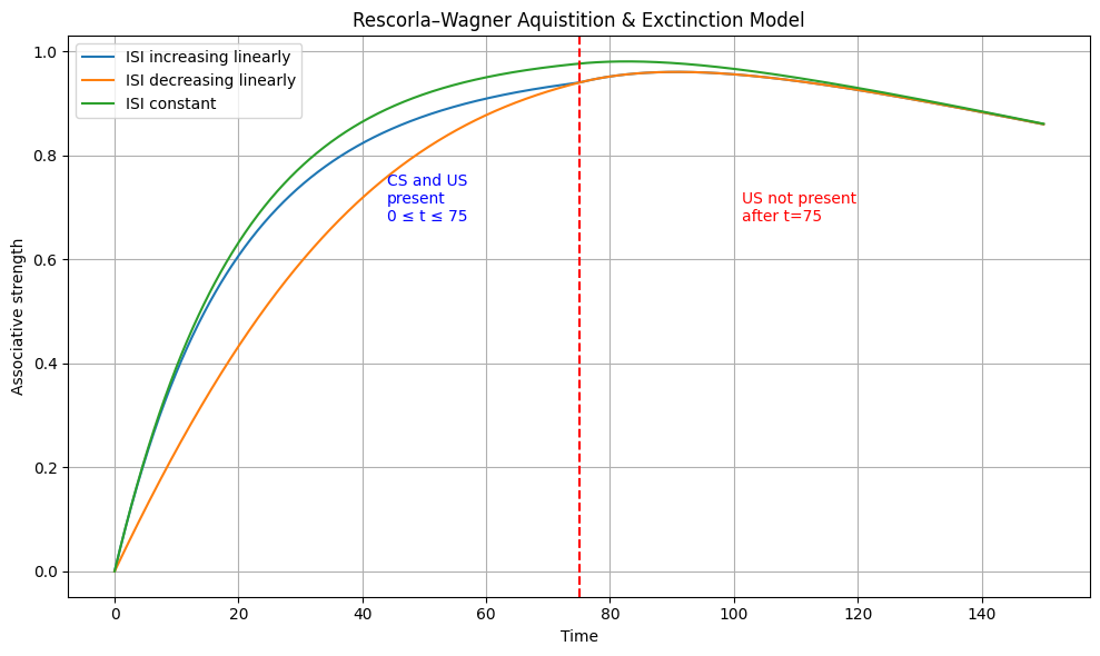
Varying the ISI over time provides a view into how it affects both acquisition and extinction. Figure 4 shows that by increasing ISI over time, acquisition starts off fast and then accelerates. Decreasing ISI over time has the opposite effect, and holding ISI constant predicatly places a curve between the two. Once extinction begins, ISI is no longer relevant, and all associative strength curves converge.

Figure 4. Updated version of the Recsorla-Wagner model considering \( ISI_{modifier} \)
4 Analysis/Conclusions
4.1 Future Improvements
Considering future work in modeling classical conditioning, we believe there are other factors to consider to provide a more accurate model. Specifically, we think it would be worthwhile to consider modeling classical conditioning outside of a vacuum. Our work considers the acquisition model in an experiment where there are no other influencing factors to alter the subject’s perception. The majority of the time, life is not governed by one controlling stimulant. Hence, it would be interesting to consider the model given the noise of other stimuli.
Further, we believe it would be worthwhile to experiment with other decay rates of the maximum associative strength, \( \lambda(t) \). Our model considers a rate that is linear. This is an initial guess we used to observe the effects \( \lambda(t) \) has on the acquisition model. It would be interesting to use other rates of decay, such as logistic decay.
It would also be intriguing to observe the model with different species for the subject. We assumed the subject to be the same for all trials. Therefore, \( \gamma \) remained the same. However, the model would change when applied to different species since the memory ability of the subjects would vary.
4.2 Notable Results
We found many fascinating results during our experiments. Notably, we found the preservation of association in the extinction model to be an exciting result. Looking at Figure 3, we observe from \( 0 \leq t < 75 \) the association represented by the blue line is considerably lower than the other two association rates. This means the subject learns the association at a much slower rate due to the saliency (\( \alpha \) ) and learning rate (\( \beta \) ). However, we see that for \( t \geq 75 \) , once the extinction is introduced, the blue line retains the association for a more extended period than the other two association rates. This implies that for retention, a slower growth in association at times is better than a fast growth.
Likewise, the results found in the ISI adaptation give interesting psychological insights into the way in which a subject forms association. We see that the associative strength grows the fastest when the timing between the bell, the CS, and the food, the US, is constant. In both cases, when we increase and decrease this timing at a linear rate, the associative strength grows at a slower rate than when the timing is constant. This provides an understanding that can be applied to classical conditioning in everyday life. For example, a teacher who wants to condition their students to be excited to do their work conditions their students using music as the CS, candy as the US, excitement (for the candy) as the UR, and excitement, once again, as the CR. From this study, the teacher knows that the fastest way to teach their kids this association is to let the timing between the music and the candy be constant every time they do the experiment. While this example is minor, there are many uses of classical conditioning and ways in which our research can be applied.
References
[1] Wikipedia contributors. (2023, October 9). Classical conditioning. Retrieved from https://en.wikipedia.org/wiki/Classical_conditioning
[2] Wikipedia contributors. (2023, February 8). Rescorla–Wagner model. Retrieved from https://en.wikipedia.org/wiki/Rescorla–Wagner_model
[3] Wilson, W. J. (2013, March). The Rescorla-Wagner Model, Simplified. Albion College.
